LLM Quantization Review

Large Language Models (LLMs) deliver impressive performance but come at the cost of high computational and memory requirements. Quantization offers a solution to mitigate these challenges by reducing memory usage and speeding up inference.

In this blog post, we’ll explore the fundamentals of quantization, the complexities specific to quantizing LLMs, and the prevailing techniques in the field. Let’s dive in.

Open Table of Contents

Motivation
Quantization Landscape
Quantization in LLM
Summary
Reference

Motivation

Deploying Large Language Models (LLMs) is both budget and energy-intensive due to their gigantic model sizes. Additionally, the cost of inference is often constrained by memory bandwith rather than math bandwidth.

Quantization offers a viable solution for mitigating the costs associated with LLMs. This technique not only minimizes GPU memory usage but also reduces the bandwidth needed for memory access. As a result, more kv caches can be accommodated within the GPU. This enables the serving of LLMs with larger batch sizes, thereby improving the compute-to-memory-access ratio.

Quantization also speeds up compute-intensive operations by representing weights and activations with low-bit integers(i.e., GEMM in linear layers, BMM in attention). For example, using 8-bit integers (INT8) can nearly double the throughput of matrix multiplications compared to using 16-bit floating-point numbers (FP16).

Quantization Landscape

In this section, we’ll delve into the fundamental concepts of quantization, covering its types, modes, and granularity.

Types of Quantization

Quantization methods fall broadly into two categories: quantization during training(QAT)¹, and post-training methods(PTQ)².

QAT incorporates the effects of quantization directly into the training process. This approach often yields higher accuracy compared to other quantization methods, as the model learns to adapt to the limitations imposed by quantization.

PTQ is applied after a model has been trained. It quantizes both the weights and activations of the model and, where possible, fuses activations into preceding layers to optimize performance.

For Large Language Models (LLMs), QAT is generally cost-prohibitive due to the computational resources required for training. As a result, PTQ is the most commonly used quantization method in the context of LLMs.

Asymmetric vs. Symmetric

Asymmetric quantization maps the range of floating-point numbers, denoted as $f_{\text{min}}/f_{\text{max}}$ , to a corresponding quantized integer range, denoted as $q_{\text{min}}/q_{\text{max}}$ . This mapping employs a zero-point (also known as quantization bias or offset) in conjunction with a scale factor, which is why it’s often referred to as zero-point quantization.

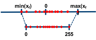
Let’s define the original floating-point tensor as $x_f$ , the quantized tensor as $x_q$ , the scale factor as $q_x$ , the zero-point as $zp_x$ , and the number of bits as $n$ . The quantization process can then be expressed as:

\begin{align}x_q &= \text{round}((x_f - \text{min}_{x_f}) * \frac{2^n - 1}{\text{max}_{x_f} - \text{min}_{x_f}}) \\ &= \text{round}(q_x x_f - \text{min}_{x_f} q_x) \\ &= \text{round}(q_xx_f - zp_x)\end{align}

Here, $q_x = \frac{2^n - 1}{\text{max}_{x_f} - \text{min}_{x_f}}$ and $zp_x = \text{min}_{x_f} * q_x$ . In practice, $zp_x$ is rounded to the nearest integer, ensuring that zero is exactly representable in the quantized range.

De-quantization reverses this process, computing $x_f$ from $x_q$ using similar equations.

Symmetric quantization, in contrast, does not map the exact $f_{\text{min}}/f_{\text{max}}$ values of the floating-point range to the quantized range. Instead, it selects the maximum absolute value between $f_{\text{min}}/f_{\text{max}}$ . Additionally, symmetric quantization does not use a zero-point. As a result, the range of values being quantized is symmetric around zero, giving this method its name: Absmax quantization.

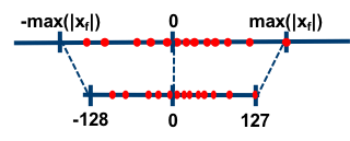
Using the same notation as before, the quantization equation becomes:

x_q = \text{round}(q_x x_f)

Here, $q_x = \frac{2^{n-1} - 1}{\text{max}(|x_f|)}$ .

When comparing these two types of quantization, symmetric quantization is simpler but comes with its own set of challenges. For instance, activations following a ReLU function are all non-negative. In such cases, symmetric quantization restricts the quantized number range to [0, 127], effectively sacrificing the precision of the second half of the range.

Granularity

Granularity refers to the extent to which parameters share the same scale factor, during the quantization process. The choice of granularity has implications for both the memory footprint and the accuracy of the quantized model.

If each parameter has its own unique scale factor, the quantization is essentially lossless. However, this approach increases the memory overhead, negating one of the primary benefits of quantization. On the other hand, if all parameters share a single scale factor, memory usage is minimized at the expense of model accuracy. In real-world applications, a balance must be struck between these two extremes.

There are typically two types of granularity: per-tensor and per-channel.

Per-tensor. This is the simplest form of granularity where all activations or weights in a tensor share the same scale factor.
Per-channel: This is a more nuanced approach, often referred to as vector-wise quantization, which includes both per-token and per-channel methods. For activations, quantization is performed along the rows, while for weights, it’s done along the columns.

Quantization in LLM

The Core Challenge

Before diving into the specifics of quantization techniques in LLM, it’s crucial to address a fundamental question: How does quantization in LLM differ from that in traditional deep learning models?

To explore this, we can use the widely-adopted 8-bit Absmax quantization as a baseline for LLM. The results of this experiment are detailed in the paper LLM.int8().

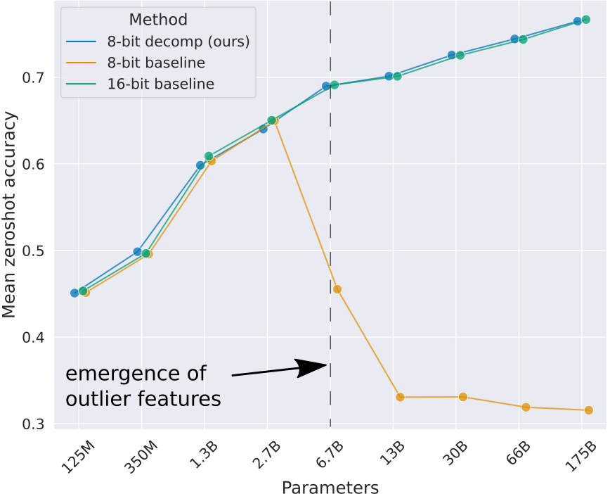
The graph includes a 16-bit baseline, which represents fp16 inference without any quantization. As evident from the data, models with sizes exceeding 6.7 billion parameters face a significant performance degradation when using the baseline quantization strategy. This highlights the need for innovative approaches to optimize quantization specifically for LLMs.

LLM.int8()

To begin, let’s analyze the root cause of the performance drop in large LLMs. The paper LLM.int8() identifies that as the model size increases, emergent features become increasingly difficult to quantize. These features manifest in specific dimensions across almost all layers and affect up to 75% of the tokens.

Consider a hidden state X in a specific transformer layer with the shape [bs, seq, hidden]. For a particular dimension index i, the values X[:, :, i] might look like:

[-60.，-45, -51, -35, -20, -67]

In contrast, 99.9% of the other dimensions have more typical values, such as:

[-0.10, -0.23, 0.08, -0.38, -0.28, -0.29, -2.11, 0.34, -0.53]

Given these disparate scales, a per-tensor quantization strategy is unsuitable. The vector-wise approach is more appropriate, specifically the per-token strategy, as previously illustrated. This choice is driven by the inefficiency of INT8 GEMM kernels when quantizing along inner dimensions.

Using per-token quantization, normal values could be adversely affected by outliers. However, these outliers are both sparse (accounting for only 0.1% of the data) and structured. In a 6.7B-parameter model, they appear in only six dimensions, represented by different i values in X[:, :, i].

Mixed-precision quantization offers a solution, allowing us to handle outliers separately.

Implementation

In this approach, the model’s parameters are stored as int8 values in DRAM. During kernel execution, the activation X identifies outliers along columns, while the weights W are decomposed accordingly along rows. Outlier features are then computed using fp16 matrix multiplication after dequantizing the weights from int8. For the remaining, “normal” activations, int8 matrix multiplication is performed first. The outputs are then de-quantized to fp16 and summed with the outlier results.

By adopting this strategy, we achieve zero degradation in accuracy. As evidenced in the figure, 8-bit decomposition yields performance nearly identical to the 16-bit baseline.

Problems

While the LLM.int8() method excels in maintaining model accuracy, it falls short in terms of computational speed, performing even slower than the 16-bit baseline. The authors have summarized the main reasons for this drawback, which can be categorized as follows:

For the release of a memory efficient implementation I needed to quickly roll a CUDA kernel for outlier extraction from matrices with a special format。 The CUDA kernel is currently not very efficient.

The fp16 matrix multiplication used in conjunction with Int8 matmul is currently run in the same CUDA stream. This makes processing sequential even though the multiplications are independent.

The fp16 matrix multiplication kernel might not be fully optimized for the extreme matrix sizes used in the outlier multiplication. A custom kernel would be lightning fast, but would require some work.

Overall, int8 matrix multiplication is not very fast for small models. This is so, because it is difficult to saturate the GPU cores with int8 elements, and as such int8 is just as fast as fp16 for small models. However, one has additional overhead of quantization which slows overall inference down.

As of now, the LLM.int8() approach has been implemented in the bitsandbytes library. Additionally, the Transformers library has integrated this quantization method.

SmoothQuant

In the realm of LLMs, there’s a general consensus that while weights are relatively straightforward to quantize, activations present challenges due to outliers. Two notable solutions have been proposed: LLM.int8() focuses on decomposing outliers for quantization, while SmoothQuant offers an alternative approach.

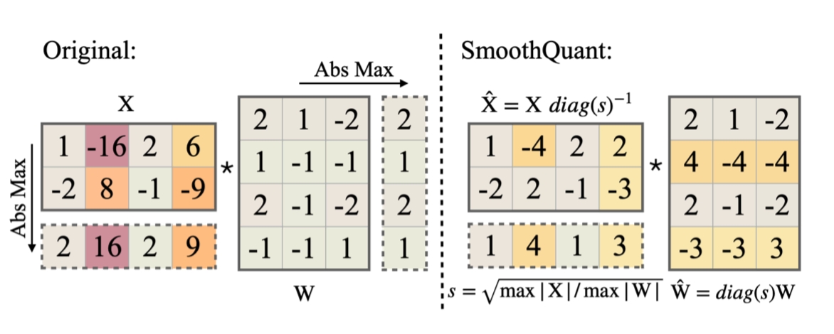
SmoothQuant aims to simplify the quantization of activations by shifting the scale variance from activations to weights. This is done offline to minimize the computational complexity during inference.

The mathematical equivalence for this operation can be expressed as:

Y = (X \text{diag}(s)^{-1}) \cdot (\text{diag}(s)W) = \hat{X} \hat{W}

Since the input X is typically the output of previous layer operations (e.g., linear layers, layer normalization, etc.), the smoothing factor can be easily fused into the parameters of these preceding layers offline, thereby avoiding any kernel call overhead.

The challenge then becomes determining an appropriate scaling factor s for quantizing $\hat{X}$ . A naive approach would be to set $s_j = \max(|X_j|), j = 1,2,\dots,C$ , ensuring that all activation channels have the same maximum value. However, this merely shifts the quantization challenge to the weights, failing to resolve the issue of accuracy degradation.

A more nuanced solution involves controlling the extent to which the quantization difficulty is transferred from activations to weights:

s_j = \max(|X_j|)^{\alpha}/\max(|W_j|)^{1-\alpha}

By judiciously selecting $\alpha$ , one can strike a balance between the difficulties associated with quantizing activations and weights.

An example with $\alpha=0.5$

GPTQ

In contrast to LLM.int8() and SmoothQuant, which aim to quantize both weights and activations, GPTQ focuses solely on weight-only quantization. It employs a one-shot, layer-by-layer approach based on approximate second-order information. For each layer, GPTQ solves the following reconstruction problem:

\argmax_{\hat{w}} = || WX - \hat{W} X||_2^2

GPTQ builds upon the Optimal Brain Quantization (OBQ) framework³, which itself is an extension of Optimal Brain Surgeon (OBS)⁴. While OBS primarily deals with sparsity and pruning, OBQ extends this concept to quantization. For a deeper dive into the mathematical derivations and code implementations, you can refer to my previous blog posts on math derivation and code explanation.

Although OBQ is theoretically sound, its computational efficiency leaves much to be desired. To address this, GPTQ introduces several engineering improvements:

Arbitrary Order: Unlike OBQ, which quantizes weights in a greedy order, GPTQ finds that the benefits of doing so are marginal. Furthermore, quantizing all rows in the same order enables parallel computation.
Lazy Batch-Updates. The straightforward implementation suffers from a low compute-to-memory-access ratio, as updating a single entry necessitates changes to the entire matrix. GPTQ mitigates this by updating elements in blocks and lazily updating subsequent parameters.
Cholesky Reformulation. To tackle numerical inaccuracies, GPTQ leverages state-of-the-art Cholesky kernels for more stable computations.

Thanks to these engineering optimizations, GPTQ can quantize a 175-billion-parameter Llama model in just 4 hours.

GPTQ employs second-order information to implicitly compensate for errors in activation outliers, offering an alternative to explicit outlier handling methods.

Activation-aware Weight Quantization(AWQ)

While GPTQ delivers impressive performance, it’s not without its drawbacks, namely overfitting on the calibration set during reconstruction and hardware inefficiency due to reordering techniques.

AWQ aims to rectify these issues by observing that not all weights are equally important. By protecting just 1% of the most salient weights, AWQ significantly reduces quantization error. Interestingly, this phenomenon—that a small subset of weights can disproportionately impact quantization error—is also observed in another research paper, SpQR.

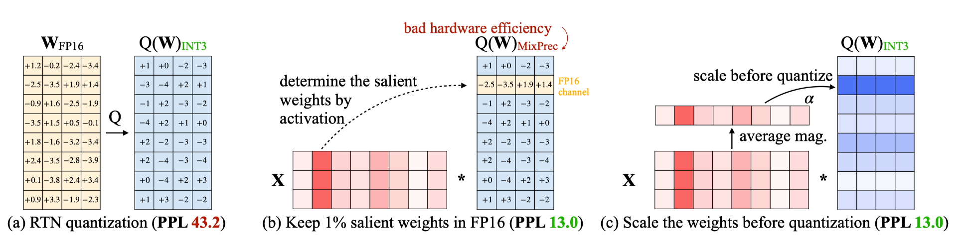
In the illustration above, the second row of weights is deemed salient due to the second column of activations. LLM.int8() (represented by diagram b) processes these salient activations separately using fp16 but suffers from computational inefficiency. SmoothQuant (diagram c) scales the weights prior to quantization.

AWQ aims to minimize the following loss function:

L(s) = ||Q(W \cdot s)(s^{-1} \cdot X) - WX||

Given that the quantization function is non-differentiable, AWQ introduces a heuristic scaling method. It decomposes the optimal scale into activation magnitude $s_X$ and weight magnitude $s_W$ as follows:

s = f(s_X, s_W) = s_X^{\alpha} \cdot s_W^{-\beta}

A simple grid search over the interval $[0, 1]$ allows for the selection of sub-optimal $\alpha$ and $\beta$ values.

AWQ closely resembles SmoothQuant, with the key difference being that AWQ focuses solely on weight quantization. For a more detailed comparison between SmoothQuant and AWQ, including code implementations, stay tuned for my upcoming blog post!

Summary

This blog post has provided an overview of the fundamental concepts of quantization, as well as a review of mainstream quantization methods in the context of LLMs. Current evidence suggests that weight-only quantization methods tend to yield better accuracy compared to methods that quantize both activations and weights. However, the challenge of effectively quantizing activations remains an open question. Successfully doing so could offer numerous benefits, such as reduced KV Cache storage and lower communication costs in tensor-parallel pattern. Research and development in this area are ongoing.

One notable issue in the current landscape is the lack of a unified benchmark for evaluating different quantization methods. Various papers employ different models like Bloom and Llama, and use different evaluation metrics, such as perplexity or test set performance. Establishing a standardized codebase could facilitate fair comparisons across methods and accelerate progress in the field.

Reference

Quantization Aware Training ↩
Post-training Quantization ↩
Optimal Brain Compression: A Framework for Accurate Post-Training Quantization and Pruning ↩
Second order derivatives for network pruning: Optimal Brain Surgeon ↩