GPTQ is a one-shot weight quantization method that leverages approximate second-order information to achieve both high accuracy and efficiency.
In this blog post, we will begin with Optimal Brain Damage (OBD)1, the foundational concept behind GPTQ, and progressively derive the mathematical theory of GPTQ.
For convenience, let’s define as a column vector, formulated as:
Next, represents the gradient matrix and is defined as:
Lastly, is the Hessian matrix, given by:
Table of Contents
Open Table of Contents
Optimal Brain Damage (OBD)1
This method employs second-order derivatives to prune weights while minimizing the impact on the network’s output. The underlying theory involves constructing a second-order approximate function to model the minimal disturbance to the local points (weights) of the objective function.
To introduce a small disturbance to the weights, we apply the Taylor Expansion to the following formula:
The change in loss due to the disturbance in is:
In the OBD paper, this equation is expressed as:
To simplify, OBD assumes that each parameter’s contribution to the loss is independent, effectively ignoring the mutual influence between parameters. This assumption is not strictly accurate but serves as an approximation.
Under this diagonal assumption, all off-diagonal elements in the Hessian matrix are zero, allowing us to simplify the equation to:
When the model has converged, the weight gradients are essentially zero (). Ignoring third-order terms, the equation further simplifies to:
This method uses second-order derivatives to assess the impact of weight disturbances on model outputs. In this local minimum, the loss is a convex function, and the second derivative is positive, meaning that weight disturbances will introduce additional errors.
The algorithm proceeds as follows:
- Build the neural network.
- Train the model until convergence.
- Compute the Hessian matrix for each weight.
- Calculate the salience of each weight.
- Sort the weights by salience, delete those with low salience, set them to zero, and freeze them.
- Repeat from step 2.
Optimal Brain Surgeon (OBS)2
While the OBD paper focuses solely on the diagonal elements of the Hessian matrix, the OBS method considers both diagonal elements and the mutual influence between parameters. The change in loss can be expressed as:
When the model has converge, we can ignore the gradients and third-order terms, simplifying the equation as follows:
Pruning the weight can be expressed as:
Here, is a unit vector where the q-th element is one, and all other elements are zeros. We can set the q-th dimension in to for pruning weights. The other dimensions in can be adjusted to balance out the errors introduced by pruning q-th dimension in .
This is a constrained optimization problem that can be solved using the Lagrange multiplier method:
Taking the derivative of with respect to and setting it to zero, we get:
From this, , substituting it into the constrained equation, we can get:
Here, represents the diagonal position with q-th element in inverse Hessian matrix, since the following equation holds.
Substituting in Equation(2), we can get:
Substituting in equation(1), the least errors introduced can be computed as:
This allows us to compute to adjust the weights and minimize the errors introduced by pruning .
The algorithm proceeds as follows:
- Train the model until convergence.
- Compute the inverse Hessian matrix .
- Iterate over all parameters and find to minimize .
- Prune and adjust weights using .
- Repeat from step 2;
The following illustration highlights the advantage of OBS over OBD:
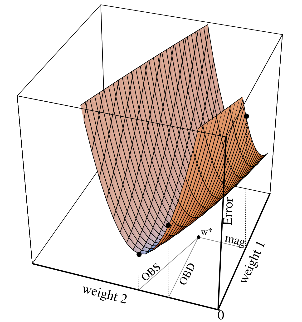
For the minimal loss weights :
- If we prune weights based on magnitude, would be pruned and set to zero, making it impossible to approach the minimum by adjusting .
- Using OBS/OBD, we can compute for both and and choose the one that minimize , allowing us to correctly prune .
- Furthermore, OBS allow us to adjust to reduce the error introduced.
Optimal Brain Compression (OBC)3
While OBS offers a more mathematically complete approach, its engineering efficiency poses a challenge.
Storing the Hessian matrix for OBS requires space, where .
Moreover, each update step has a time complexity of , leading to a total time complexity of . This is prohibitively slows for modern neural network.
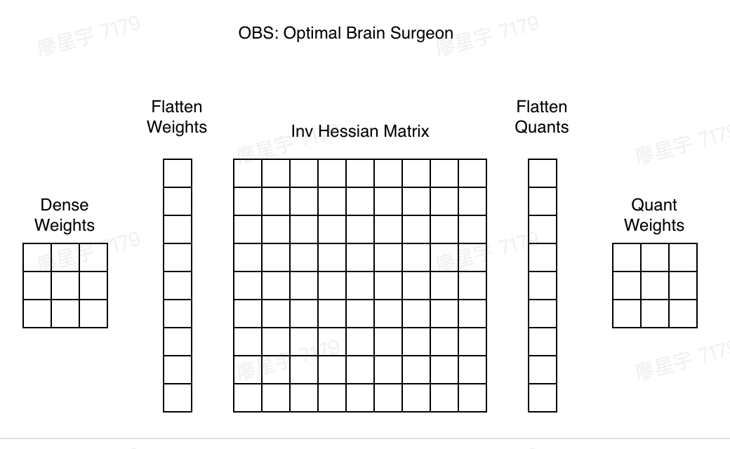
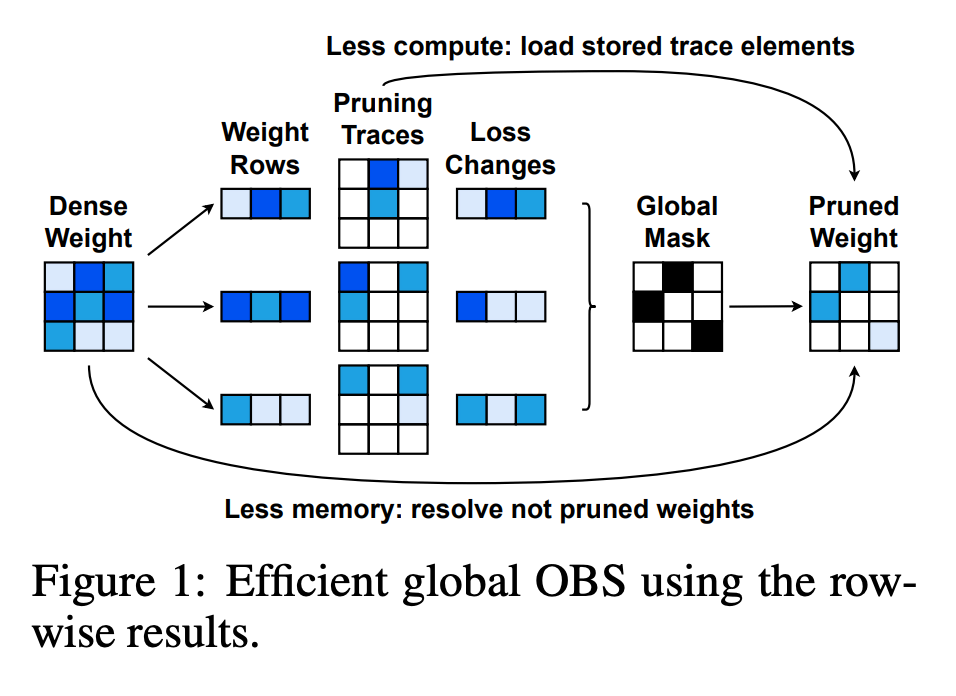
To address this, the OBC paper reformulates the objective function as:
With this formulation, pruning can be carried out along each row independently. If parameters are pruned in in each row , the time complexity can be reduced to .
Optimal Brain Quantization (OBQ)3
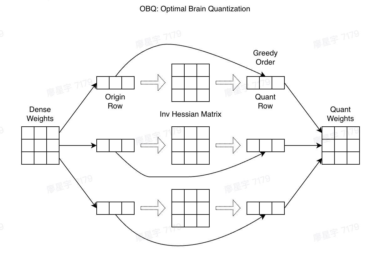
Besides pruning, the OBC paper also proposes a quantization method named OBQ, as pruning can be considered a special form of quantization (quantizing parameters to zero).
The OBQ method can be derived by modifying the OBC constraints as follows:
By substituting for , the quantization equations can be computed as:
In the same way as OBC, quantization for each row can be carried out independently. The time complexity is since all parameters needs to be quantized.
GPTQ
Although OBQ has improved computational efficiency, it’s still not suitable for Large Language Models (LLMs). GPTQ comes to the rescue, further boosting efficiency with the following main optimizations:
Use arbitrary order instead of greedy one
The OBQ paper always picks the weights which currently incurs the least additional errors. But the GPTQ paper finds that greedy order’s improvement over quantizing weights in arbitrary order is small.
The original OBQ method quantizes rows of independently with a specific order defined by corresponding errors. But in GPTQ, all rows can be quantized with the same order. As a consequence, each column can be quantized at one time.
In this way, the runtime can reduce from to .
Lazy Batch-Updates
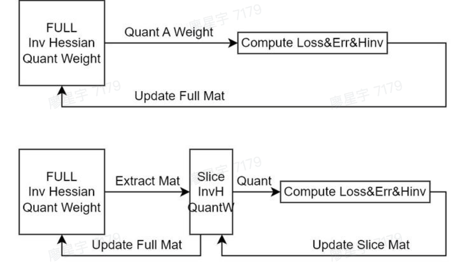
In OBQ, quantizing a single element requires updating all elements using the following equation:
This lead to a relatively low compute-to-memory-access ratio. For example, if the weight matrix is and quantizing is done along columns, the total memory-access IO is .
Fortunately, this problem can be resolved by the following observation: The final rounding decisions for column i are only affected by updates performed on this very column, and so updates to later columns are irrelevant at this point in the process.
This makes it possible for “lazily batch” updates for later parameters together, thus achieving much better GPU utilization.
Cholesky Reformulation
The inverse of Hessian computations has numerical stability problem when scaling GPTQ to existing models.
Except for applying dampening, that is adding a small constant to diagonal elements, leverage state-of-the-art Cholesky kernels to compute all information we will need from upfront.
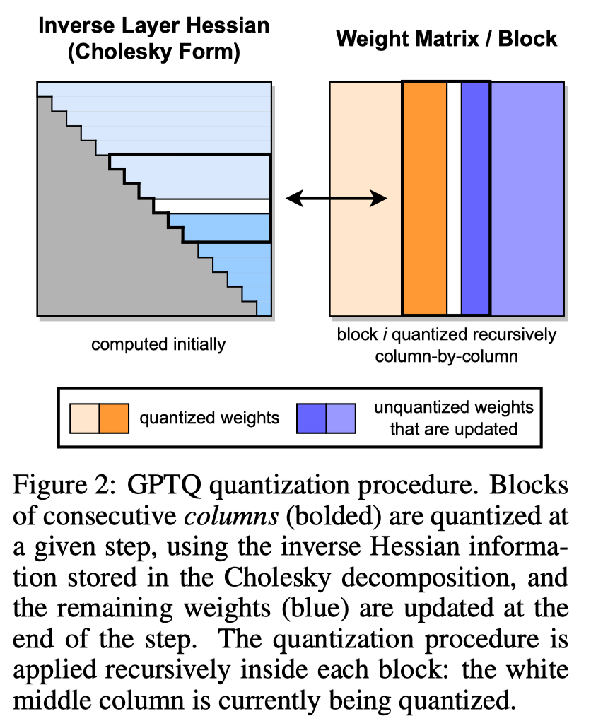
GPTQ proceeds as follows:
- Compute the upfront.
- Split the elements into multiple blocks.
- Quantize each block along columns.
- Update the elements in this block.
- Repeat step 3 if there are more blocks.
Summary
This blog post traces the development of GPTQ, starting from its roots in OBD, through OBS, and finally to OBC. Unlike quantization methods based on statistical approaches, GPTQ is grounded in rigorous theoretical proof, making it a more robust and reliable solution.
What’s Next?
This blog post has covered the theoretical underpinnings of GPTQ, and in the upcoming post, we will get hands dirty with the code implementation.
Stay tuned for a deep dive into the code that powers this fascinating approach to weight quantization!