This is the third blogpost of Triton tutorial series.
In this tutorial, we will write a high-performance matrix multiplication kernel that achieves performance on parallel with cuBLAS step by step.
Motivations
General Matrix Multiplications (GEMMs)1 serve as a cornerstone for numerous operations in Large Language Models (LLMs), including self-attention and fully-connected layers. However, writing and optimizing GEMMs can be a daunting task. Hence their implementation is generally done by hardward vendors as part of so-called “kernel libraries”, such as cuBLAS.
While implementing matrix multiplication requires a strong background in High-Performance Computing (HPC), GEMMs must also be easily customizable to meet the unique demands of modern deep learning workloads. These demands often include fused activation functions and quantization techniques.
To give you an idea of what we’re dealing with, let’s consider the following blocked algorithm. This algorithm multiplies a matrix of dimensions (M, K) by another matrix of dimensions (K, N):
# Do in parallel
for m in range(0, M, BLOCK_SIZE_M):
  # Do in parallel
  for n in range(0, N, BLOCK_SIZE_N):
    acc = zeros((BLOCK_SIZE_M, BLOCK_SIZE_N), dtype=float32)
    for k in range(0, K, BLOCK_SIZE_K):
      a = A[m : m+BLOCK_SIZE_M, k : k+BLOCK_SIZE_K]
      b = B[k : k+BLOCK_SIZE_K, n : n+BLOCK_SIZE_N]
      acc += dot(a, b)
    C[m : m+BLOCK_SIZE_M, n : n+BLOCK_SIZE_N] = acc
In this algorithm, each iteration of the doubly-nested for-loop is executed by a dedicated Triton program instance.

Naive GEMM
In this section, we’ll present the first version of our Triton implementation for the GEMM algorithm discussed earlier. One of the main challenges lies in calculating the memory locations where blocks of matrices A and B should be read during the inner loop. This requires a deep understanding of multi-dimensional pointer arithmetic.
Understanding Pointer Arithmetic
In a row-major 2D tensor x, the memory location of X[i, j] can be calculated as &X[i, j] = &X + i * stride_xi + j * stride_xj. Using this formula, we can define the blocks of pointers for A[m : m+BLOCK_SIZE_M, k : k+BLOCK_SIZE_K] and B[k : k+BLOCK_SIZE_K, n : n+BLOCK_SIZE_N] in pseudo-code as follows:
&A[m : m+BLOCK_SIZE_M, k : k+BLOCK_SIZE_K] = a_ptr + (m : m+BLOCK_SIZE_M)[:, None]*A.stride(0) + (k : k+BLOCK_SIZE_K)[None, :]*A.stride(1);
&B[k : k+BLOCK_SIZE_K, n : n+BLOCK_SIZE_N] = b_ptr + (k : k+BLOCK_SIZE_K)[:, None]*B.stride(0) + (n : n+BLOCK_SIZE_N)[None, :]*B.stride(1);
Here, we employ the broadcasting mechanism to compute the data block index.
Triton Code for Pointer Arithmetic
In Triton, we can use the pid along with dimensions M and N to calculate the pointer for blocks of A and B. The code snippet below illustrates this:
pid = triton.program_id(0);
grid_m = (M + BLOCK_SIZE_M - 1) // BLOCK_SIZE_M;
grid_n = (N + BLOCK_SIZE_N - 1) // BLOCK_SIZE_N;
pid_m = pid / grid_n;
pid_n = pid % grid_n;
Here, grid_m and grid_n represent the number of programs along each dimension. The total number of programs is grid_m * grid_n, as each row block in A needs to be computed with all column blocks in B. The variables pid_m and pid_n serve as the starting data indices in A and B for a given pid.
After determining the data block indices, we can proceed to calculate the data pointers for A and B:
offs_am = (pid_m * BLOCK_SIZE_M + tl.arange(0, BLOCK_SIZE_M)) % M
offs_bn = (pid_n * BLOCK_SIZE_N + tl.arange(0, BLOCK_SIZE_N)) % N
offs_k = tl.arange(0, BLOCK_SIZE_K)
a_ptrs = a_ptr + (offs_am[:, None] * stride_am + offs_k[None, :] * stride_ak)
b_ptrs = b_ptr + (offs_k[:, None] * stride_bk + offs_bn[None, :] * stride_bn)
It’s worth noting that we need to include an extra modulo operation to handle cases where M is not a multiple of BLOCK_SIZE_M or N is not a multiple of BLOCK_SIZE_N. In such scenarios, we can pad the data with zeros so that they do not contribute to the final results.
With this consideration, the pointers for blocks of A and B can be updated in the inner loop as follows:
a_ptrs += BLOCK_SIZE_K * stride_ak
b_ptrs += BLOCK_SIZE_K * stride_bk
Inner Computations
Once we have the pointers for the data blocks of matrices A and B, the next step is to compute the corresponding block in the output matrix C. To prevent overflow, we accumulate the results into a [BLOCK_SIZE_M, BLOCK_SIZE_N] block of fp32.
We run a for-loop along the K dimension, processing BLOCK_SIZE_K elements in each iteration. To ensure we’re within bounds, we generate a mask based on the current value of K.
# offs_k = tl.arange(0, BLOCK_SIZE_K)
for k in range(0, tl.cdiv(K, BLOCK_SIZE_K))
	a = tl.load(a_ptrs, mask=offs_k[None, :] < K - k * BLOCK_SIZE_K, other=0.0)
	b = tl.load(b_ptrs, mask=offs_k[:, None] < K - k * BLOCK_SIZE_K, other=0.0)
After loading the essential data blocks, we carry out the matrix multiplication and accumulate the results in accumulator. It’s important to note that we use float32 for the accumulator to prevent overflow issues that could arise with float16 matmul (Matrix Multiplication).
# accumulator = tl.zeros((BLOCK_SIZE_M, BLOCK_SIZE_N), dtype=tl.float32)

accumulator += tl.dot(a, b)

a_ptrs += BLOCK_SIZE_K * stride_ak
b_ptrs += BLOCK_SIZE_K * stride_bk
Finally, we write the computed block back to the output matrix C. We use pointer arithmetic similar to the data loading step, but this time we also include a mask to ensure we’re within the bounds of C.
offs_cm = pid_m * BLOCK_SIZE_M + tl.arange(0, BLOCK_SIZE_M)
offs_cn = pid_n * BLOCK_SIZE_N + tl.arange(0, BLOCK_SIZE_N)
c_ptrs = c_ptr + (offs_cm[:, None] * stride_cm + offs_cn[None, :] * stride_cn)
c_mask = (offs_cm[:, None] < M) & (offs_cn[None, :] < N)
tl.store(c_ptrs, accumulator, mask=c_mask)
Here is the full code:
@triton.jit
def matmul_kernel_naive(
    a_ptr,
    b_ptr,
    c_ptr,
    M,
    N,
    K,
    stride_am,
    stride_ak,
    stride_bk,
    stride_bn,
    stride_cm,
    stride_cn,
    BLOCK_SIZE_M: tl.constexpr,
    BLOCK_SIZE_N: tl.constexpr,
    BLOCK_SIZE_K: tl.constexpr,
):
    pid = tl.program_id(0)

    # get size of pid by m-axis and n-axis
    num_pid_m = (M + BLOCK_SIZE_M - 1) // BLOCK_SIZE_M
    num_pid_n = (N + BLOCK_SIZE_N - 1) // BLOCK_SIZE_N
    pid_m = pid // num_pid_n
    pid_n = pid % num_pid_n

    # get start and end index
    offs_am = (pid_m * BLOCK_SIZE_M + tl.arange(0, BLOCK_SIZE_M)) % M
    offs_bn = (pid_n * BLOCK_SIZE_N + tl.arange(0, BLOCK_SIZE_N)) % N
    offs_k = tl.arange(0, BLOCK_SIZE_K)

    # do pointer arithmetic for data loading
    # 2d block
    a_ptrs = a_ptr + (offs_am[:, None] * stride_am + offs_k[None, :] * stride_ak)
    b_ptrs = b_ptr + (offs_k[:, None] * stride_bk + offs_bn[None, :] * stride_bn)

    accumulator = tl.zeros((BLOCK_SIZE_M, BLOCK_SIZE_N), dtype=tl.float32)
    for k in range(0, tl.cdiv(K, BLOCK_SIZE_K)):
        # load data
        a_data = tl.load(
            a_ptrs, mask=offs_k[None, :] < (K - k * BLOCK_SIZE_K), other=0.0
        )
        b_data = tl.load(
            b_ptrs, mask=offs_k[:, None] < (K - k * BLOCK_SIZE_K), other=0.0
        )

        # execute computation
        accumulator += tl.dot(a_data, b_data)

        # Advanced pointers to next K block
        a_ptrs += BLOCK_SIZE_K * stride_ak
        b_ptrs += BLOCK_SIZE_K * stride_bk

    accumulator = accumulator.to(dtype=tl.float16)
    # write back the block of output matrix with masks
    offs_cm = pid_m * BLOCK_SIZE_M + tl.arange(0, BLOCK_SIZE_M)
    offs_cn = pid_n * BLOCK_SIZE_N + tl.arange(0, BLOCK_SIZE_N)
    c_ptrs = c_ptr + (offs_cm[:, None] * stride_cm + offs_cn[None, :] * stride_cn)
    c_mask = (offs_cm[:, None] < M) & (offs_cn[None, :] < N)
    tl.store(c_ptrs, accumulator, mask=c_mask)
L2 Cache Optimization
In the naive version, each program instance calculates a [BLOCK_SIZE_M, BLOCK_SIZE_N] block of the matrix C. It’s crucial to note that the sequence in which these blocks are computed has an impact on the L2 cache hit rate of our program.
To illustrate, recall the naive row-major ordering defined as follows:
pid = triton.program_id(0);
grid_m = (M + BLOCK_SIZE_M - 1) // BLOCK_SIZE_M;
grid_n = (N + BLOCK_SIZE_N - 1) // BLOCK_SIZE_N;
pid_m = pid / grid_n;
pid_n = pid % grid_n;
For example, if each matrix consists of 9x9 blocks, the naive version (using row-major ordering) would require loading 90 blocks into SRAM to compute the first 9 output blocks. In contrast, an optimized approach would only need to load 54 blocks.

This optimized approach enhances data reuse by ‘super-grouping’ blocks in sets of GROUP_M rows before moving on to the next column. The code snippet below illustrates this:
# Program ID
pid = tl.program_id(axis=0)
num_pid_m = tl.cdiv(M, BLOCK_SIZE_M)
num_pid_n = tl.cdiv(N, BLOCK_SIZE_N)

# Number of programs in group
num_pid_in_group = GROUP_SIZE_M * num_pid_n
# Id of the group this program is in
group_id = pid // num_pid_in_group

# Row-id of the first program in the group
first_pid_m = group_id * GROUP_SIZE_M
# If `num_pid_m` isn't divisible by `GROUP_SIZE_M`, the last group is smaller
group_size_m = min(num_pid_m - first_pid_m, GROUP_SIZE_M)

# *Within groups*, programs are ordered in a column-major order
# Row-id of the program in the *launch grid*
pid_m = first_pid_m + (pid % group_size_m)
# Col-id of the program in the *launch grid*
pid_n = (pid % num_pid_in_group) // group_size_m
Here, we first calculate the number of program IDs (pids) along the M and N dimensions. Then we determine the number of pids in each GROUP_SIZE_M and the group ID for each pid. Next, we identify the first pid in each group. Finally, we compute the column-major ordered pid_m and pid_n.
Hyperparameters AutoTuning
Selecting the optimal hyperparameters for your kernel, such as BLOCK_SIZE_M, BLOCK_SIZE_N, and BLOCK_SIZE_K, can be a challenging task. Different combinations can significantly impact performance, especially across various hardware platforms.
A naive approach would be to manually try different sets of hyperparameters. However, Triton simplifies this process by providing an API called triton.autotune.
Here’s a straightforward example demonstrating how to employ autotune:
@triton.autotune(
    configs=[
        triton.Config({'BLOCK_SIZE_M': 128, 'BLOCK_SIZE_N': 256, 'BLOCK_SIZE_K': 64, 'GROUP_SIZE_M': 8}, num_stages=3, num_warps=8),
        triton.Config({'BLOCK_SIZE_M': 64, 'BLOCK_SIZE_N': 256, 'BLOCK_SIZE_K': 32, 'GROUP_SIZE_M': 8}, num_stages=4, num_warps=4),
        triton.Config({'BLOCK_SIZE_M': 128, 'BLOCK_SIZE_N': 128, 'BLOCK_SIZE_K': 32, 'GROUP_SIZE_M': 8}, num_stages=4, num_warps=4)
    ],
    key=['M', 'N', 'K'],
)
@triton.jit
def matmul_kernel(...,
		M, N, K,
		...
    BLOCK_SIZE_M: tl.constexpr,
    BLOCK_SIZE_N: tl.constexpr,
    BLOCK_SIZE_K: tl.constexpr,
    GROUP_SIZE_M: tl.constexpr,
)
The triton.autotune is a Python decorator that can be applied directly to the kernel function. The configs parameter specifies different combinations of hyperparameters. The num_stages and num_warps options control the compiler’s behavior for software pipelining and parallelization2, respectively. The key parameter lists the argument names that, when changed, will trigger a reevaluation of all provided configurations.
After the autotuning process, the best-performing kernel configuration is cached. When the same input shapes are encountered again, the cached configuration is used, thereby speeding up execution. It’s common practice to “warm up” the autotuner before deploying the model for inference.
Performance can be benchmarked using methods discussed in the previous tutorial.
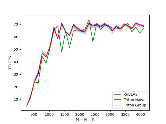
As seen in the graph, the grouped version slightly outperforms the naive one, and both are nearly as efficient as the cuBLAS version.
In the next tutorial, we will extend the gemm operation to batched gemm and introduce how to use the Nsight system for kernel performance profiling, offering more detailed insights.
Stay tuned!
Reference
- Triton Tutorials: Matrix Multiplication
- OpenAI/Triton MLIR 第二章: Batch GEMM benchmark
- Matrix Multiplication Background User’s Guide