In the realm of Large Language Models (LLMs), various quantization methods exist for inference, including LLM.int8, GPTQ, and SmoothQuant. This blog post will specifically focus on SmoothQuant and its enhanced counterpart, AWQ. These methods are designed to tackle the feature emergence problem that often arises in LLMs.
We’ll start by examining the challenges associated with quantizing LLMs. Then, we’ll dive into the intricacies of both SmoothQuant and AWQ, highlighting their differences and unique advantages. At last, we will explore the code implementation of these methods.
Table of Contents
Open Table of Contents
Intro
As Large Language Models (LLMs) continue to grow in size, scaling from 7 billion to 70 billion parameters, the importance of quantization techniques has never been more pronounced. Quantization not only enables us to fit large models like a 30-billion-parameter model onto consumer-grade GPUs such as the 4090, but it also effectively reduces IO bandwidth, a critical consideration given that LLMs inference is often more memory-bound than compute-bound.
For those interested in a broader overview of quantization and its role in LLMs, you can refer to my previous blog post, LLM Quantization Review. That post also introduces the basic concepts behind SmoothQuant and AWQ.
In this blog, we will delve deeper into SmoothQuant and its enhanced version(I call it), AWQ. Our focus will be on the details of quantization process.
Review of Quantization Difficulty
Activation Outliers
In SmoothQuant, the authors note that when scaling Large Language Models (LLMs) beyond 6.7 billion parameters, systematic outliers with large magnitudes begin to appear in activations. These outliers pose a significant challenge to activation quantization.
Similarly, AWQ observes that not all weights are equally important; protecting just 1% of salient weights can significantly reduce quantization error. Actually, these 1% salient weights often correspond to the outliers in activations.
Another key observation is that these outliers tend to persist in fixed channels, showed in below, constituting a small fraction of the total channels. This aligns with the 1% salient weights identified in AWQ.

Given the specific pattern of activation outliers, per-tensor quantization becomes impractical. For vector-wise quantization, two schemes exist: per-token and per-channel.

While per-token quantization has little impact, per-channel quantization proves to be effective, as confirmed by experimental results in SmoothQuant.

Limitations in Scheme
Although per-channel quantization preserves model accuracy, it is not compatible with INT8 GEMM kernels. In these kernels, scaling can only be performed along the outer dimensions of the matrix multiplication, such as the token dimension of activations and the output channel dimension of weights. This scaling is typically applied after the matrix multiplication is complete.
Given the complexities surrounding activation outliers and the limitations of existing quantization schemes, it’s crucial to understand how SmoothQuant and AWQ navigate these challenges. Let’s delve into their respective approaches.
SmoothQuant and AWQ
The Approach
While per-channel quantization is highly effective, it’s not feasible for certain computational kernels. To address this, SmoothQuant proposes “smoothing” the input activation by dividing it by a per-channel smoothing factor . To maintain the mathematical equivalence of a linear layer, the weights are scaled in the opposite direction:
On the other hand, AWQ focuses on selecting salient weights based on activation magnitudes to improve performance. By scaling up these salient weight channels, quantization error can be significantly reduced. The optimization objective for AWQ is:
Interestingly, despite their different motivations, both SmoothQuant and AWQ arrive at the same quantization formula. This formula involves per-channel scaling in input activations and inner channel scaling in weights.
Determining the Scaling Factors
A critical aspect of the quantization process is the choice of the scaling factor .
In SmoothQuant, the scaling factor is determined to balance the quantization difficulty between activations and weights, making both easier to quantize. The formula for is as follows:
Here, serves as a hyper-parameter that controls how much difficulty is shifted from activations to weights. For instance, setting yields the following example:
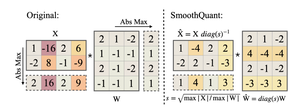
In this example, the maximum absolute values for each channel in activation and each input dimension in weights are computed using AbsMax. The scaling factor is then calculated using the above formula with . The “smoothed” activation and weight are both easy to quantize after this smoothing process.
AWQ also decomposes the scaling factor into components related to activation magnitude and weight magnitude:
Unlike SmoothQuant, AWQ determines the optimal values for and through a simple grid search over the interval . Besides, and is the average magnitude, which means and .
Difference
While SmoothQuant and AWQ may appear similar due to their equations, they differ in some aspects.
In SmoothQuant, the “smoothed” activations are quantized and then involved in INT8 matrix multiplication with the weights. Below is a diagram illustrating the precision mapping for a single Transformer block in this method:

Contrastingly, AWQ is a weight-only quantization method. It relies on the magnitude of activations to identify salient weights, which are then preserved through scaling. This can also be interpreted as a way to preserve outlier activations. In AWQ, all matrix multiplications in the Transformer block are performed at fp16 precision, as the weights are dequantized from fixed-point numbers.
Code Impl.
Having explored the fundamental principles of quantization in SmoothQuant and AWQ, let’s now delve into their code implementations.
The implementation can be broadly categorized into two main components: the quantization process and the quantized kernel implementation. We’ll start by discussing the quantization process before moving on to the kernel implementation.
SmoothQuant
In SmoothQuant, the first step involves determining the scales for activations. The core function for this is get_act_scales, which can be found here.
The key component is the forward_hook, where x represents the input activations. The function stat_tensor selects the maximum absolute values across all channels and stores these statistics for later use.
def get_act_scales(model, tokenizer, dataset_path, num_samples=512, seq_len=512):
    ...
    def stat_tensor(name, tensor):
        hidden_dim = tensor.shape[-1]
        tensor = tensor.view(-1, hidden_dim).abs().detach()
        comming_max = torch.max(tensor, dim=0)[0].float().cpu()
        if name in act_scales:
            act_scales[name] = torch.max(act_scales[name], comming_max)
        else:
            act_scales[name] = comming_max

    def stat_input_hook(m, x, y, name):
        if isinstance(x, tuple):
            x = x[0]
        stat_tensor(name, x)

    hooks = []
    for name, m in model.named_modules():
        if isinstance(m, nn.Linear):
            hooks.append(
                m.register_forward_hook(
                    functools.partial(stat_input_hook, name=name))
            )
    ...
    return act_scales
After determining the maximum absolute value for each activation channel, we need to find the corresponding maximum value in the weights to compute the scales. The function smooth_ln_fcs accomplishes this task.
@torch.no_grad()
def smooth_ln_fcs(ln, fcs, act_scales, alpha=0.5):
    ...
    weight_scales = torch.cat([fc.weight.abs().max(
        dim=0, keepdim=True)[0] for fc in fcs], dim=0)
    weight_scales = weight_scales.max(dim=0)[0].clamp(min=1e-5)

    scales = (act_scales.pow(alpha) / weight_scales.pow(1-alpha)
              ).clamp(min=1e-5).to(device).to(dtype)

    ln.weight.div_(scales)
    ln.bias.div_(scales)

    for fc in fcs:
        fc.weight.mul_(scales.view(1, -1))
Here, ln represents LayerNorm and fcs are the linear layers following LayerNorm. There are multiple such layers, like Q, K, V, after the first LayerNorm in the attention mechanism.
weight_scales represents the maximum absolute values along the inner dimension of the weights. Note that this value is the maximum taken across all linear layers and is clamped to a minimum of 1e-5. Subsequently, the scales are computed using both act_scales and weight_scales. Finally, these activation scales are fused into the preceding LayerNorm layer, while the weight scales are applied to modify the weights of all linear layers.
After “smoothing” the activations and weights, the function get_static_decoder_layer_scales is used to collect the scales for the inputs and outputs of the linear layers, which will be used for quantizing the activations.
@torch.no_grad()
def get_static_decoder_layer_scales(model,
                                    tokenizer,
                                    dataset_path,
                                    num_samples=512,
                                    seq_len=512,
                                    ):
    ...
    def stat_io_hook(m, x, y, name):
        if isinstance(x, tuple):
            x = x[0]
        if name not in act_dict or "input" not in act_dict[name]:
            act_dict[name]["input"] = x.detach().abs().max().item()
        else:
            act_dict[name]["input"] = max(
                act_dict[name]["input"], x.detach().abs().max().item())
        if isinstance(y, tuple):
            y = y[0]
        if name not in act_dict or "output" not in act_dict[name]:
            act_dict[name]["output"] = y.detach().abs().max().item()
        else:
            act_dict[name]["output"] = max(
                act_dict[name]["output"], y.detach().abs().max().item())
    ...
Register stat_io_hook for all linear layers and collect the absolute maximum value across all elements in inputs and outputs activations.
Finally, the quantized model is generated with the following line:
int8_model = Int8OPTForCausalLM.from_float(model, decoder_layer_scales)The from_float function is recursively invoked on the submodules, resulting in a final set of quantized layers that include LayerNormQ, W8A8B8O8LinearReLU, and W8A8BFP32OFP32Linear. Additionally, the quantized batched matrix multiplication operations are performed using BMM_S8T_S8N_F32T and BMM_S8T_S8N_S8T. These components will be discussed in detail in the subsequent blog on quantized kernels.
AWQ
AWQ shares many similarities with SmoothQuant, and the core quantization process is encapsulated in the function run_awq. This function can be broadly categorized into three main steps:
- Acquire decoder layers and calibration set;
- Determine scales for activations and weights, and apply them;
- Identify the clipping range for weights and implement it.
The first part is self-explanatory, so let’s focus on the second part concerning scale determination.
Scaling
The function auto_scale_block is central to finding scales, and within it, _search_module_scale employs grid search to identify the optimal scale ratio. Let’s break down _search_module_scale.
Initially, scales for weights and activations must be determined. The variable linears2scale contains all linear layers to be quantized in this block for the same input activations. For instance, in self_attention, the layers q_proj, k_proj, and v_proj all operate on the same input.
Concatenating all linear weights allows us to find w_max using get_weight_scale. If q_group_size > 0, weights are reshaped by [-1, q_group_size] because each q_group_size will share the same scales. Subsequently, weights are normalized to [0, 1] and the mean is computed along the output channels as the weight base scale.
Finding the activation scale is straightforward, as there’s only one. The code snippet below illustrates this:
@torch.no_grad()
def get_act_scale(x):
    return x.abs().view(-1, x.shape[-1]).mean(0)

@torch.no_grad()
def get_weight_scale(weight, q_group_size=-1):
    org_shape = weight.shape
    if q_group_size > 0:
        weight = weight.view(-1, q_group_size)
    scale = weight.abs() / weight.abs().amax(dim=1, keepdim=True)
    scale = scale.view(org_shape)
    scale = scale.mean(0)
    return scale

# self attention as example
linear2scale = [module.self_attn.q_proj, module.self_attn.k_proj, module.self_attn.v_proj]

# w: co, ci
weight = torch.cat([_m.weight for _m in linears2scale], dim=0)
w_max = get_weight_scale(
    weight, q_group_size=q_config.get("q_group_size", -1))
The final step involves a grid search for the best scales. The original output, org_out, is obtained by invoking the forward function of the original block for error measurement.
x = x.to(next(block.parameters()).device)
with torch.no_grad():
    org_out = block(x, **kwargs)
    if isinstance(org_out, tuple):
        org_out = org_out[0]
A for-loop iterates through all grid points, computing the corresponding scales. The square root of the product of the max and min values serves as a form of geometric mean between these two extremes.
for ratio in range(n_grid):
    ratio = ratio * 1 / n_grid
    scales = (x_max.pow(ratio) / w_max.pow(1-ratio)
              ).clamp(min=1e-4).view(-1)
    scales = scales / (scales.max() * scales.min()).sqrt()
To simulate the real computation process, weights are multiplied by scales and subjected to pseudo-quantization. Activations are divided by scales, which is equivalent to dividing the scales on new pseudo-quantized weights.
for fc in linears2scale:
		fc.weight.mul_(scales.view(1, -1).to(fc.weight.device))
    fc.weight.data = w_quantize_func(
        fc.weight.data) / (scales.view(1, -1))
After this, we obtain the de-quantized weights corresponding to the scales. We can then compute the errors introduced by scaling and quantization. The best hyperparameters are easily selected through grid search.
out = block(x, **kwargs)
if isinstance(out, tuple):
    out = out[0]

loss = (org_out - out).float().pow(2).mean().item()  # float prevents overflow
history.append(loss)
is_best = loss < best_error
Finally, scales are applied to weights and activations. As previously mentioned, activation scales can be fused into the preceding layer. There are three types of layers before a linear: linear, layernorm, and activation. The code snippets below show how to apply scales to these layers.
@torch.no_grad()
def scale_fc_fc(fc1, fc2, scales):
    ...
    fc1.weight[-scales.size(0):].div_(scales.view(-1, 1))
    fc2.weight.mul_(scales.view(1, -1))
    ...

@torch.no_grad()
def scale_ln_fcs(ln, fcs, scales):
    ...
    if not isinstance(fcs, list):
        fcs = [fcs]

    ln.weight.div_(scales)
    if hasattr(ln, 'bias') and ln.bias is not None:
        ln.bias.div_(scales)

    for fc in fcs:
        fc.weight.mul_(scales.view(1, -1))
    ...
For activations that don’t have weights to fuse, a new forward method must be defined. This is accomplished using the ScaledActivation wrapper class. The wrapper takes the original activation function as an argument and applies the scales directly during the forward pass.
class ScaledActivation(nn.Module):
    def __init__(self, module, scales):
        super().__init__()
        self.act = module
        self.scales = nn.Parameter(scales.data)

    def forward(self, x):
        return self.act(x) / self.scales.view(1, 1, -1).to(x.device)
Lastly, if input activations are provided, scales are also applied to them for later clipping use. This avoids the need for re-computation using scaled weights.
# apply the scaling to input feat if given; prepare it for clipping
if input_feat_dict is not None:
    for layer_name in layer_names:
        inp = input_feat_dict[layer_name]
        inp.div_(scales.view(1, -1).to(inp.device))
Clipping
This section serves as a supplementary part, focusing on clipping weights to a reasonable range to minimize errors. The core function for this operation is auto_clip_layer.
Firstly, both inputs and weights are reshaped to account for the group_size used in quantization. The shapes are transformed as follows: [n_token, ci] -> [1, n_token, n_group, group_size] for inputs and [co, ci] -> [co, 1, n_group, group_size] for weights.
group_size = q_config["q_group_size"] if q_config["q_group_size"] > 0 else w.shape[1]
input_feat = input_feat.view(-1, input_feat.shape[-1])
input_feat = input_feat.reshape(1, input_feat.shape[0], -1, group_size)
input_feat = input_feat[:, 0::input_feat.shape[1] // n_sample_token]
w = w.reshape(w.shape[0], 1, -1, group_size)
To prevent out-of-memory (OOM) errors, each iteration selects a sub-weight slice for computation, denoted as w = w_all[i_b * oc_batch_size: (i_b + 1) * oc_batch_size].
The absolute maximum value of the weight along group_size in the input channel is computed as org_max_val = w.abs().amax(dim=-1, keepdim=True). A grid search is then employed to determine the optimal max_value for clipping weights. Due to the group_size, torch.matmul cannot be used. Instead, shape expansion, element-wise multiplication, and sum reduction are used to simulate the matmul operation, although this requires more GPU memory.
The clipping process is straightforward: iterate through all possible max_val, clip the weights accordingly, apply pseudo-quantization, and run the forward pass to obtain outputs. These outputs are then compared with the original to find the max_val that minimizes error.
# input_feat: [1, n_token, n_group, group_size]
# w: [co_i, 1, n_group, group_size]

org_out = (input_feat * w).sum(dim=-1)  # co, n_token, n_group
for i_s in range(int(max_shrink * n_grid)):
    max_val = org_max_val * (1 - i_s / n_grid)
    min_val = - max_val
    cur_w = torch.clamp(w, min_val, max_val)
    q_w = pseudo_quantize_tensor(cur_w, n_bit=n_bit, **q_config)
    cur_out = (input_feat * q_w).sum(dim=-1)

    err = (cur_out - org_out).pow(2).mean(dim=1).view(min_errs.shape)
    ...
After identifying the optimal max_val, applying it to clip the weights is a simple task.
for name, max_val in clip_list:
    layer = get_op_by_name(module, name)
    layer.cuda()
    max_val = max_val.to(layer.weight.device)
    org_shape = layer.weight.shape
    layer.weight.data = layer.weight.data.reshape(*max_val.shape[:2], -1)
    layer.weight.data = torch.clamp(layer.weight.data, -max_val, max_val)
    layer.weight.data = layer.weight.data.reshape(org_shape)
    layer.cpu()
Summary
This blog post revisits the challenges associated with LLM quantization and delves into two closely related methods: SmoothQuant and AWQ. These methods address the feature emergence problem by “smoothing” activations and scaling weights. The post also provides a detailed walkthrough of the code implementation behind the quantization processes of these methods.
However, this is not the final word on these quantization techniques. An important discussion on quantized kernels awaits us. Stay tuned for the next blog post, where we will explore the implementation of quantized kernels!